Topic Modeling in Python – Discover how to Identify Top N Topics

Identifying top research topics from a large volume of data is a skill to have as a data analyst or data scientist. This will help you know the trend in the topic from your datasets or research area. Therefore, you are going to discover how to do topic modeling in python. Hence, this will help you to identify top N topics from any hidden structures in collections of text. In this paper, we shall explore how to build and run this model with a tutorial

Topic Modeling in Python:

Firstly, topic Modeling simply explained is a technique used to extract hidden topics from a large dataset of text. There are different algorithms used for topic modeling in python but however, the Latent Dirichlet Allocation (LDA) remains the popular algorithm for topic modeling. Furthermore, this is implemented in this work using the genism package. However, extracting good quality topics depends heavily on the quality of datasets and the number of topics. Therefore in this tutorial, you will learn how to implement the LDA algorithm for topic modeling in python

1. Introduction

In this paragraph, I am going to describe how to analyze a large volume of text from tweets, emails, social media comments, or research papers. Imagine this problem as on your task as a result of being a data analyst//scientist. Hence, one of the ways to achieve this is through Natural Language Processing (NLP). The NLP is the process of manipulating natural language like speech and text using the software. Moreover, this enables us to have a proper understanding of problems, opinions that are valuable to businesses, government policies, administrators, and others

Moreover, this cannot be done manually. It requires an automated algorithm that reads through the large volume of text and automatically gives the output of the topic discovered.

Therefore, in this tutorial, I will walk you through how to identify top N_topics using a transportation dataset. We shall use the LDA to extract these identified topics. Also, we shall be able to visualize these topics using PyLDavis and Wordcloud. Therefore, LET US BEGIN

2. Task Definition and Scope

Our task in this project is to identify the top 25 research topics for Transportation Research Part B between 2010 and 2017 from the Trid Website.

3. MUST DO! Installation of Important Packages

The first approach to starting this task is to firstly, go to the Trid Website and download the datasets. I know you can do this. However, if you cannot, you can click here to download the dataset using our GitHub clone. The next step is to read the datasets on our jupyter notebook using python. Hence, to do this, you need to install these packages.

import numpy as np
import pandas as pd
import datetime
import matplotlib.pyplot as plt
%matplotlib inline
!pip install RISparser
from RISparser import readris
from RISparser.config import TAG_KEY_MAPPING

From the above, we imported pandas, numpy, matplotlib and rispsarser. Since our dataset is stored with xxxxx.ris, we shall be needing these packages : from RISparser import readris. This will enable us to read the data. Note, if you run into errors with the packages, simply use !pip install #then the package name.

Moreover, we shall install these packages such as NLTK, spacy, re, PyLDavis, and wordcloud.

!pip install tqdm 
import nltk
nltk.download('punkt')
nltk.download('stopwords')
nltk.download('wordnet')
from nltk.tokenize import word_tokenize
from nltk.stem.wordnet import WordNetLemmatizer
import spacy

import re


#Importing of Genism --Gensim is a free open-source Python library used to represent documents as semantic vectors, as efficiently (computer-wise) and painlessly (human-wise) as possible.
import gensim
import gensim.corpora as corpora
from gensim.utils import simple_preprocess
from gensim.models import CoherenceModel

#Importing some plotting tools to aid in visualisation
!pip install pyLDAvis
import pyLDAvis
import pyLDAvis.gensim_models as gensimvis
pyLDAvis.enable_notebook()  # don't skip this


#Importing WordCloud
from wordcloud import WordCloud, STOPWORDS
import matplotlib.colors as mcolors


import warnings
warnings.filterwarnings("ignore",category=DeprecationWarning)

Therefore, the above shows the complete packages we will use in this tutorial. However, I will try to explain what each of these packages does when we shall be using them.

4. Loading, Cleaning and Data Wrangling of the dataset

In this section, we will load our data on our IDE. Firstly, remember we stored our file as .ris. Hence, you shall learn how to read ris files in python. We shall clone the file from Github using the code below. This will make it available to all.

!git clone https://github.com/JOHNPAUL-ADIMS/Research-Topic-Modelling-with-LDA.git

Furthermore, the code as shown below will open and read the file from the file path.

#Reading my ris file
filepath = '/content/Research-Topic-Modelling-with-LDA/TRIDRIS_2022-02-26.ris'

mapping = TAG_KEY_MAPPING
mapping["SP"] = "pages_this_is_my_fun"
with open(filepath, 'r') as bibliography_file:
  entries = list(readris(bibliography_file, mapping=mapping))

The next thing for us is to convert this file to a data frame. To do this, we shall be use pandas.

  # converting the dictionary to a dataframe
  df = pd.DataFrame.from_dict(entries) 
 
  #checking out for the top rows
  display(df.head())

Shown below, is the out:

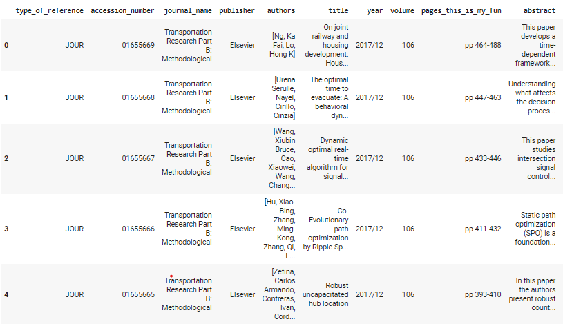
We can also perform some cleaning and wrangling processes of our data.

df.info() #This obtains the data informations. It also shows us the columns avaiable and their type

Below is the outcome of the code.

<class 'pandas.core.frame.DataFrame'>
RangeIndex: 1078 entries, 0 to 1077
Data columns (total 15 columns):
 #   Column                Non-Null Count  Dtype 
---  ------                --------------  ----- 
 0   type_of_reference     1078 non-null   object
 1   accession_number      1078 non-null   object
 2   journal_name          1078 non-null   object
 3   publisher             1078 non-null   object
 4   authors               1078 non-null   object
 5   title                 1078 non-null   object
 6   year                  1078 non-null   object
 7   volume                1078 non-null   object
 8   pages_this_is_my_fun  1078 non-null   object
 9   abstract              1077 non-null   object
 10  keywords              1078 non-null   object
 11  type_of_work          1077 non-null   object
 12  doi                   832 non-null    object
 13  url                   1078 non-null   object
 14  number                292 non-null    object
dtypes: object(15)
memory usage: 126.5+ KB

From the above, we shall see that there are rows with missing data. Hence we shall use remove them using isnull and dropna.

# Checking out for a a cell with no abstract content
df['abstract'].isnull().sum()

# Removing cell with no article
df.dropna(subset = ["abstract"], inplace=True)
transport_topics = df  #The new DataFrame

Converting year to date time on python

transport_topics['year'] = pd.to_datetime(transport_topics['year'])

# extracting the year from the datetype
transport_topics['Year']= df['year'] = pd.DatetimeIndex(transport_topics['year']).year

# Finding the number of articles published in different years
publish_date = transport_topics['Year'].value_counts()
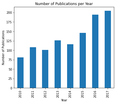
publish_date

Visualizing number of publications per year

In this, we used matplotlib to make our visualization.

# Visualizing the number of publications per year
date_pub = df.groupby(transport_topics['Year'])['abstract'].count()
date_pub.plot(kind='bar', 
              title='Number of Publications per Year', 
              ylabel='Number of Publications',
              xlabel='Year', 
              figsize=(6, 5)
              )

5. Data preparation for topic modeling in python.

For the sake of this tutorial, we shall use abstracts for topic modeling in python. Once we have established this, we need to get our data ready to be consumed by the LDA model. The first thing is to remove symbols in the abstract. To do this you shall use the code below:

#Removing symbols from Abstracts
transport_topics['Abstract_Cleaned'] = transport_topics.apply(lambda row: (re.sub("[^A-Za-z0-9' ]+"," ", str(row['abstract']))),axis=1)

After, we shall implement tokenization, stopwords, bigrams, trigrams, and finally lemmatize it.

# Tokenization 
transport_topics['Abstract_Cleaned']= transport_topics.apply(lambda row: (word_tokenize(str(row['Abstract_Cleaned']))), axis = 1)

# Running the Stopwords
stopwords = stopwords.words("english")
stop_words = set(stopwords)
transport_topics['Abstract_Cleaned'] = transport_topics.apply(lambda row: ([w for w in row['Abstract_Cleaned'] if w not in stop_words]),axis=1)


# Lemmatization
lementize = WordNetLemmatizer()
df2 = transport_topics.apply(lambda row: ([lementize .lemmatize(w) for w in row['Abstract_Cleaned']]), axis=1)

Creating Bigram and Trigram for topic modeling in python

Bigrams and trigrams help remove words that are made up of two or three characters. An N-gram is a contiguous sequence of n items from a given sample of text or speech

The code below creates the bigram and trigram model.

bigram = gensim.models.Phrases(df2,
                               min_count=5, #This defines the minimum time the words needs to occur to be considered as bigram
                               threshold=1000) # The higher threshold fewer phrases.

trigram = gensim.models.Phrases(bigram[df2], threshold=100)


# Creating an object 
bigram_mod = gensim.models.phrases.Phraser(bigram)
trigram_mod = gensim.models.phrases.Phraser(trigram)

# defining the functions stopwords, bigrams and trigrams
def remove_stopwords(texts):
    return [[word for word in simple_preprocess(str(doc)) if word not in stop_words] for doc in texts]

def make_bigrams(texts):
    return([bigram[doc] for doc in texts])

def make_trigrams(texts):
    return ([trigram[bigram[doc]] for doc in texts])

def lemmatization(texts, allowed_postags=['NOUN', 'ADJ', 'VERB', 'ADV']):
    """https://spacy.io/api/annotation"""
    texts_out = []
    for sent in texts:
        doc = nlp(" ".join(sent)) 
        texts_out.append([token.lemma_ for token in doc if token.pos_ in allowed_postags])
    return texts_out

# Removing of Stop Words
data_words_nostops = remove_stopwords(df2)

# Forming of trigrams
data_words_trigrams = make_trigrams(data_words_nostops)

# Initialize spacy 'en' model, keeping only tagger component (for efficiency)
# python3 -m spacy download en
nlp = spacy.load('en', disable=['parser', 'ner'])

# Do lemmatization keeping only noun, adj, vb, adv
data_lemmatized = lemmatization(data_words_trigrams, allowed_postags=['NOUN', 'ADJ', 'VERB', 'ADV'])

6. Latent Dirichlet Allocation Model

LDA stands for Latent Dirichlet Allocation This is a type of topic modeling algorithm. The purpose of LDA is to learn the representation of a fixed number of topics, and given this number of topics learn the topic distribution that each document in a collection of documents has

Before creating the LDA model, we need to create a dictionary that will contain our cleaned abstract.

# Creating Dictionary and Corpus
dictionary = corpora.Dictionary(data_lemmatized)
texts = data_lemmatized
corpus = [dictionary.doc2bow(text) for text in data_lemmatized]

Implementing Gensim will help create a unique id for each of the words in the document. Hence, let’s build our LDA model using Genism.

# Building LDA Model
lda_model = gensim.models.ldamodel.LdaModel(corpus=corpus,
                                           id2word=dictionary,
                                           num_topics=25, #Identifies the 25 topic trends for transportation
                                           random_state=100,
                                           update_every=1,
                                           chunksize=100,
                                           passes=10,
                                           alpha='auto',
                                           per_word_topics=True)

doc_lda = lda_model[corpus]

From the model above we were able to make our N topics to be 25. alpha and eta are hyperparameters that affect the sparsity of the topics. According to the Gensim docs, both default to 1.0/num_topics prior. chunksize is the number of documents to be used in each training chunk. update_every determines how often the model parameters should be updated and passes is the total number of training passes.

However, to see the distribution of the keywords use the code below:

# Printing of the keywords in the topics
pprint(lda_model.show_topics(formatted=False))

[(13,
  [('source', 0.06512987),
   ('trade', 0.045173783),
   ('site', 0.040406674),
   ('mechanism', 0.0329754),
   ('panel', 0.031640574),
   ('reference', 0.02912658),
   ('hypothetical', 0.026253037),
   ('loss', 0.024065124),
   ('limitation', 0.019442359),
   ('psychological', 0.017859435)]),
 (11,
  [('stop', 0.09174625),
   ('charge', 0.053283878),
   ('station', 0.052258007),
   ('infrastructure', 0.031791538),
   ('wait', 0.026819773),
   ('action', 0.02056839),
   ('waiting', 0.020266762),
   ('line', 0.019517427),
   ('battery', 0.01874809),
   ('metaheuristic', 0.017555248)]),
 (7,
  [('parking', 0.072828494),
   ('signal', 0.061196424),
   ('lane', 0.056751538),
   ('cycle', 0.03909413),
   ('intersection', 0.033130523),
   ('delay', 0.020027665),
   ('traffic', 0.018675707),
   ('discharge', 0.014754855),
   ('control', 0.013961559),
   ('group', 0.013459547)]),
 (15,
  [('datum', 0.052678652),
   ('information', 0.051902752),
   ('segment', 0.046523623),
   ('measurement', 0.02880827),
   ('method', 0.027260905),
   ('maintenance', 0.025540648),
   ('estimation', 0.023030333),
   ('pavement', 0.020984298),
   ('calibration', 0.018633153),
   ('probe', 0.017169837)]),
 (17,
  [('frequency', 0.065366775),
   ('speed', 0.048180413),
   ('hub', 0.038067717),
   ('service', 0.03152919),
   ('line', 0.031468384),
   ('variance', 0.028742988),
   ('meeting', 0.023522481),
   ('operator', 0.021250341),
   ('threshold', 0.021233056),
   ('energy', 0.021115456)]),
 (20,
  [('traffic', 0.1061415),
   ('flow', 0.045046095),
   ('vehicle', 0.026612155),
   ('density', 0.019469857),
   ('model', 0.019083543),
   ('driver', 0.017460773),
   ('oscillation', 0.013770127),
   ('speed', 0.013297865),
   ('behavior', 0.012972597),
   ('condition', 0.0125916945)]),
 (0,
  [('problem', 0.091247536),
   ('solution', 0.05107057),
   ('propose', 0.041792747),
   ('design', 0.031716954),
   ('solve', 0.030912064),
   ('level', 0.020295016),
   ('cost', 0.020097483),
   ('method', 0.019152755),
   ('base', 0.018237581),
   ('algorithm', 0.017138612)]),
 (9,
  [('model', 0.05530292),
   ('use', 0.030271294),
   ('choice', 0.02682107),
   ('estimate', 0.020272397),
   ('datum', 0.019178415),
   ('distribution', 0.016726132),
   ('result', 0.01595804),
   ('approach', 0.011984581),
   ('paper', 0.01152869),
   ('estimation', 0.011434947)]),
 (21,
  [('network', 0.060031734),
   ('model', 0.052648816),
   ('link', 0.026618497),
   ('author', 0.025516775),
   ('flow', 0.018552195),
   ('base', 0.015195785),
   ('path', 0.014616386),
   ('present', 0.013736709),
   ('first', 0.0132576395),
   ('paper', 0.0124428915)]),
 (16,
  [('time', 0.07161434),
   ('author', 0.03077816),
   ('travel', 0.030082744),
   ('model', 0.029472776),
   ('system', 0.020908358),
   ('use', 0.017381975),
   ('demand', 0.01575878),
   ('show', 0.013979408),
   ('case', 0.012420036),
   ('value', 0.01121222)])]

7. Computation of Model Perplexity and Coherence Score

Model Perplexity and Coherence Score are used to check for the accuracy of the trained model. This model is helpful.

# Compute Perplexity Score
print('The Perplexity Score is : ', lda_model.log_perplexity(corpus))  # This measures of how good the model is. The lower the better.

# Compute Coherence Score
coherence_model_lda = CoherenceModel(model=lda_model, texts=data_lemmatized, dictionary=corpora.Dictionary(data_lemmatized), coherence='c_v')
coherence_lda = coherence_model_lda.get_coherence()
print('The Coherence Score is : ', coherence_lda)

8. Data Visualization

We shall be visualizing our data using PyLDavis and WordCloud.

PyLDavis Visualization for Topic Modeling in Python

vis = pyLDAvis.gensim_models.prepare(lda_model, 
                                     corpus, 
                                     dictionary, 
                                     mds="mmds", 
                                     R=20) #This choses the number of word a topic should contain.
vis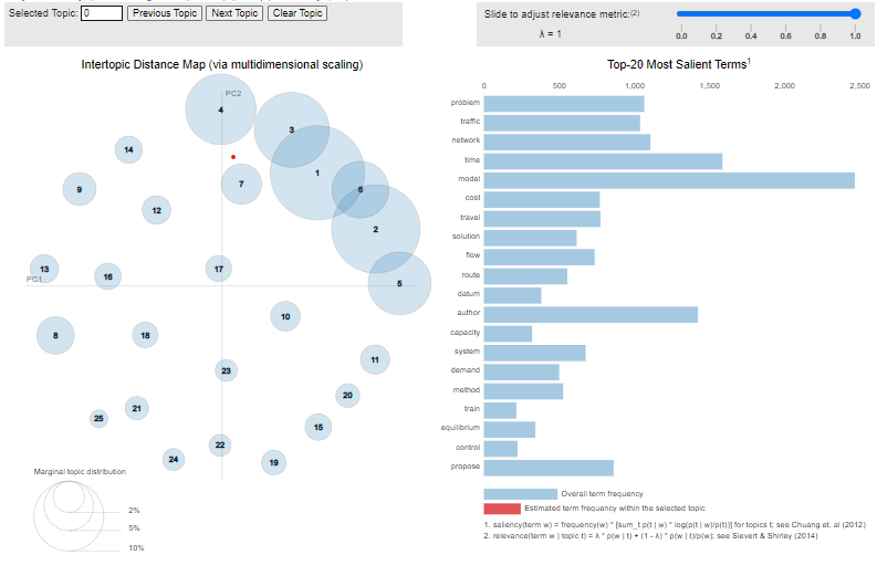

From the above PyLDavis output, we can infer the following:

The bigger bubbles on the left side show the more important topics.

For a good topic model, it will have fairly big, non-overlapping bubbles scattered throughout the edge of the quadrant instead of clustering in one quadrant.

On the right hand, we can see the words and the bars. When you hover the cursor on any bubbles, the right-hand words will update. These silent keywords are formed from the selected topic. You can enter the topic number you want to see from the select topic tab.

WordCloud Visualization

Our next visualization of the model is the word cloud. Since we are able to identify top N_topics from our dataset, we are going to visualize our model’s result on the word cloud. We shall arrange this in n-rows and n -columns.

cloud = WordCloud(stopwords=stop_words,
                  background_color='white',
                  prefer_horizontal=1,
                  height=330,
                  max_words=200,
                  colormap='flag',
                  collocations=True)

topics = lda_model.show_topics(formatted=False)

fig, axes = plt.subplots(5, 5, figsize=(10,10), sharex=True, sharey=True)

for i, ax in enumerate(axes.flatten()):
    fig.add_subplot(ax)
    plt.imshow(cloud.fit_words(dict(lda_model.show_topic(i, 200))))
    plt.gca().set_title('Topic' + str(i), fontdict=dict(size=12))
    plt.gca().axis('off')


plt.subplots_adjust(wspace=0, hspace=0)
plt.axis('off')
plt.suptitle("The Top 25 Research Topic Trend for Transportation Research Part B", 
             y=1.05,
             fontsize=18,
             fontweight='bold'
             )
plt.margins(x=0, y=0)
plt.tight_layout()
plt.show()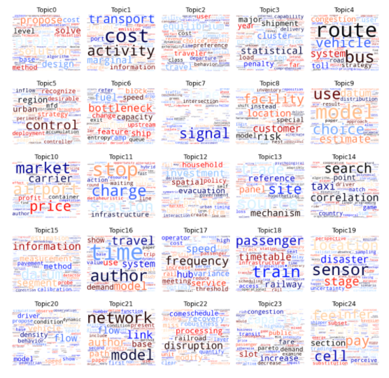

From the above, we can infer the following topics :

1. Topic 0 – Transportation Problems, and Proposes Possible solution.
2. Topic 1 – Transportation Cost Analysis.
3. Topic 2 – Mode of Transportation among Travellers
4. Topic 3 – Logistics and Supply Chain
5. Topic 4 – Transportation Route
6. Topic 5 – Transportation Networks, Control and Strategy
7. Topic 7 – Traffic Management
8. Topic 8 – Transportation Hub
9. Topic 9 – Transportation Modelling
10. Topic 10 – Air Transportation and Airline Management
11. Topic 11 – Transport Fare Mangagement System
12. Topic 12 – Transportation Policies and Investments
13. Topic 14 – Taxi Transportation
14. Topic 15 – Maintenance and Information System
15. Topic 17 – Rail Transportation
16. Topic 18 – Rail Transportation Infastructure
17. Topic 19 – Transportation Disaster and Uncertainity Management
18. Topic 20 – Traffic Congestion Optimization and Management
19. Topic 21 – Modelling and Network System
20. Topic 22 – Transportation Disruption and Recovery
21. Topic 23 – Capacity Building to easy Congestion
22. Topic 24 – Financial- Payment Method

Conculsion

From the identified top 25 topics, we can see that researchers are focused on the 3 modes of transportation i.e. air, land, and water. However, land transportation has more dominance over research activities. These research activities are in the area of traffic congestions, transport fare, infrastructure amongst others. There is also research on air transportation, railway, and sea.

The results of this topic modeling can also be improved. This can be done by increasing the number of topics during the LDA modeling.